LLM Inference Benchmarking - Measure What Matters

Production-grade LLM inference is a complex systems challenge, requiring deep co-designs - from hardware primitives (FLOPs, memory bandwidth, and interconnects) to sophisticated software layers - across the entire stack. Given the hardware variability across GPU providers like NVIDIA and AMD - including generational differences in numeric type performance (FP8, BF16, NVFP4 etc), HBM bandwidth and capacity, peak FLOPs etc - optimal performance is never guaranteed. It depends on the software’s ability to maximize FLOPs utilization during prefill, maximize bandwidth efficiency during decode, optimize expert routing in MoE models, discovering optimal parallelism strategies, and more.

As inference hardware costs remain high, squeezing maximum performance to improve unit economics is a primary objective for AI teams. We are currently in an era of intense hardware-software co-design that will redefine performance and cost efficiency. Consequently, benchmarking must evolve to track three critical pillars: end-to-end model performance, micro-benchmarking of isolated components and a structured way to go after performance improvements. This article focuses on the LLM performance domain and analyzes the interplay between latency, throughput, concurrency, and cost.

Prefill and Decode: The two phases of Inference

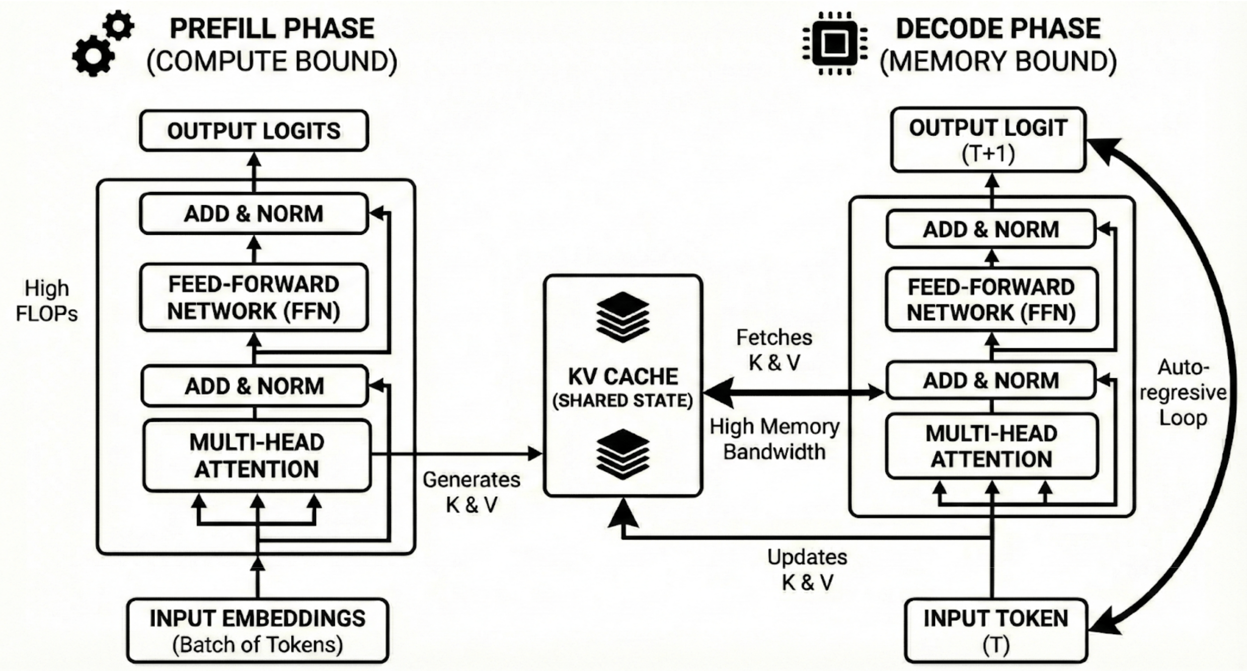
LLM Inference works in two-phases: prefill and decode. The prefill phase is where the entire input goes through the model’s forward pass which includes self-attention, add & norm, and pass through the hidden layers of the model’s feed forward network. This phase is extremely compute bound. FLOPs per byte transferred (arithmetic intensity) for the prefill phase is very high. In simpler terms, the GPU is spending more time computing than waiting for the data from memory.

On the other hand, the decode phase is memory bound. For every token that is generated, decode needs to load the entire weight matrix, KV cache from the HBM, generate one token, and write it back to the HBM to compute the next token. GPUs end up spending more time waiting for data from the memory than spending time in computation. These two phases, thus, have very different computation characteristics.

Metrics

In this section, we’ll go through several metrics that have a direct impact on the user perception of Inference performance.

Time to First Token (TTFT)

Time to First Token is a key metric that measures the duration between when a prompt is submitted to when the model generates its first token. From a user standpoint, this is the “waiting” time from submitting a prompt to seeing the text stream.

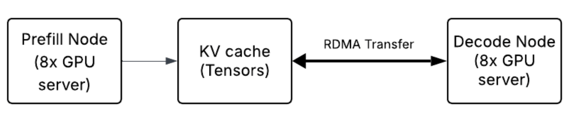
TTFT is closely tied to the prefill phase as the model cannot start generating any token until the entire forward-pass from the input sequence (prompt) is done and the initial KV cache is populated. Maximizing arithmetic intensity (FLOPS per byte transferred), optimal attention (MHA, MLA, GQA) kernels, memory bandwidth efficiency (e.g. FlashAttention), optimal linear layers, activation kernels, and optimal batch scheduling are the hallmarks of optimizing the prefill phase which has a direct impact on TTFT. In disaggregated setups, where prefill and decode are separated across network boundaries (for example, RDMA across 8x servers), KV cache transfer latency from prefill to decode workers impact TTFT depending on the orchestration strategy. For example - some implementations generate the first token from the prefill worker before or while the KV cache is being transferred to the decode worker. In those implementations, the transfer affects the latency of the second token (ITL), but not the TTFT itself.

Time per Output Token (TPOT)

Time per Output Token measures how fast the text flows once it starts streaming. This is calculated as an end-to-end metric, stripping out the TTFT from end-to-end latency and dividing by the total number of tokens generated from the remaining intervals . TPOT, thus provides an overall perception of text flow speed to the end user. Depending on the use case, text flowing too slowly or too fast may not be an ideal experience for an end-user.

ITL = (E2E - TTFT) / (N - 1)

While TTFT is tied to the prefill phase, TPOT is a good proxy to the performance of the decode phase. Decode is strictly memory-bound and happens one-token at a time (unlike the prefill phase). Each new token requires the model to load the entire model weight matrix and KV cache from the GPU HBM, generate the token and write back the KV cache to GPU HBM. TPOT is therefore limited by the memory bandwidth of the GPU. As an example - AMD MI355X (HBM bandwidth of 8 TB/s) will have a better TPOT than AMD MI325X (HBM bandwidth of 6 TB/s).

Inter Token Latency (ITL)

Inter Token Latency is often confused with TPOT but there is a subtle difference. While TPOT is an end-to-end metric, ITL strictly measures the time lapse between two consecutive tokens (e.g. time between Tn+1 and Tn). ITL is a useful metric to both measure the decode throughput as well as variance. High variance in ITL is not ideal as it signals jitter in token generation, which to an end user feels like text now flowing smoothly. While ITL is also a decode phase metric, it is a bit lower level and helps in measuring jitters in decode performance that may be caused for several reasons like 1) Interference from large prefill operations monopolizing the FLOPs, 2) System going through PagedAttention, 3) Sub-optimal hardware topology setup (e.g. cross NUMA domain traffic) and other kernel level in-efficiencies.

End to End Latency (E2EL)

End to End latency is a measure of the duration of a request from a user. For example, if a user sent a 1K (ISL) prompt to the model and is expecting 8K (OSL) response, then E2EL measures the duration between the first byte sent from the user to the last byte of the last token received by the user. E2EL is therefore an aggregate metric that is somewhat calculated as below:

E2EL = Network Overhead + TTFT + (TPOT * Number of Tokens)

E2EL is a useful metric for real time inference workloads where every millisecond counts. For example, E2EL for a model hosted in North America for a user in close proximity will be much smaller than for a user accessing a model from across the Atlantic. Other factors that may impact E2EL are request queuing, tokenization overhead, and so on.

Token Throughput (TPS)

Token Throughput measures the total number of tokens generated by the inference system per second across all active user requests. This is different from what request throughput is supposed to measure, for example, token throughput can be really high for decode heavy (large OSL) workloads but RPS could be modest. TPS is a good utilization proxy, it is easy to do some back of the envelope math to calculate the “speed of light” generation throughput i.e. what’s the maximum throughput you can get from the hardware if everything else (kernels, software etc) worked perfectly. Decode has to load the entire model weights + KV cache from the HBM to compute the next tokens iteratively one-by-one. Therefore, speed of light throughput, roughly can be calculated:

Single Request TPSsol = Bandwidth / Data Moved

which translates in specific terms to:

Single Request TPSsol = HBM Bandwidth / (Model Weights + (Context Length * KV bytes per token))

Model weights refers to bytes per parameter (e.g. 2 bytes for FP16, 1 byte for FP8). KV bytes per token depends on specific model architecture (num_layers, heads, dimensions, precision).

The above formula is for concurrency (C=1). Modeling for higher concurrency can be done in a similar way (with some nuances) by adding concurrency factors to the equation. This gives a good “limit of silicon” frontier measure as the north star (keep in mind that TPSsol decays as the context length grows).

Request Throughput (RPS)

Request Throughput measures how many end to end user requests are handled by the inference system per unit of time - seconds, minutes etc. RPS is a good proxy for how many tasks or users are being served by the system. RPS is typically increased by handling more requests in parallel. For example, if you send 1 request at a time sequentially, the GPU is spending most of its time idling and to get more out of the hardware, you let it do more work in parallel. However, there is a limit to which you can load the system with parallel requests, beyond which the latency metrics as discussed above start getting affected. Ultimately, there is a peak of request throughput tied to the limits of the silicon and it is worth modeling what is the speed of light (SoL) RPS that can be achieved on specific hardware. Modeling RPS speed of light is a bit more nuanced, as it requires accounting for non-linear interaction between prefill compute and decode memory access.

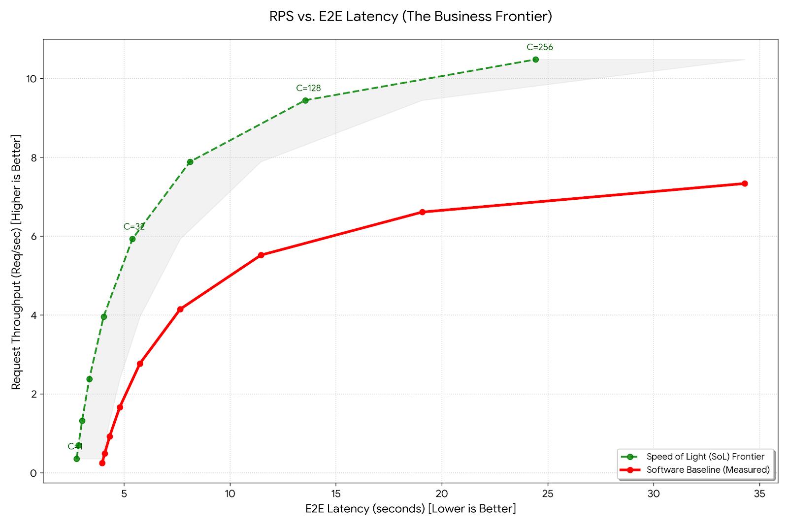
The Pareto Frontier

Now that we understand the foundational set of inference metrics, it is worth noting that there is a complex interplay between the throughput and latency metrics with constant trade-offs between the two. Moreover, layer in the request density and you end up with several dimensions to optimize for. There are three main vectors that are in constant tension: latency, throughput, and concurrency. If you optimize for latency alone, your cost-per-token suffers, if you optimize for throughput alone, latency suffers. Without a framework, it soon becomes a game of “whack-a-mole”. If foundational metrics give you a picture of where you are, the Pareto frontier provides a picture of where you can be.

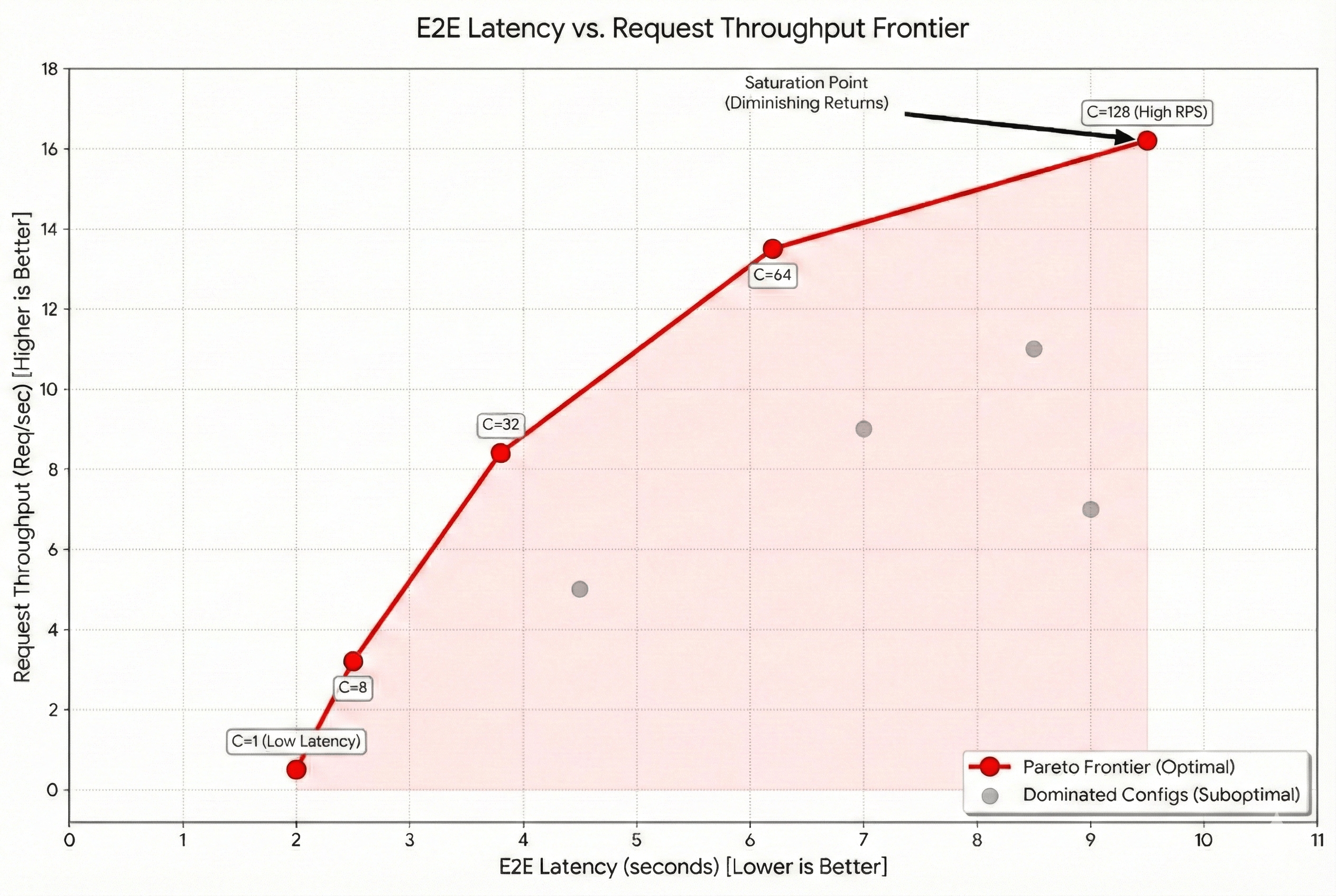
The frontier graph above tracks request throughput against e2e latency on a concurrency surface. By adding more concurrent requests to the workload, we attempt to increase the throughput. However, increasing the concurrency has an impact on negatively affecting the e2e latency. The graph above shows an example frontier for a 1-128 concurrency sweep. Frontier is the ideal “discovered” configuration and it is usually a good idea to start with the baseline frontier and optimize from there. For example, any configs that are below and right of the frontier do not meet the minimum bar and can be discarded. A general step-by-step checklist is helpful while starting any benchmarking effort:

Step 1: Establish a baseline Pareto frontier

With our experience with character.ai and other inference customers, we know that any production-grade AI Inference workload is trying to optimize a specific workload and the shape of the workload is usually definitions of:

1. Which model to use
2. ISL / OSL ratio
3. Target latency while optimizing cost

Cost is determined on how much request density can be packed on a per unit server (e.g. 1X H100 or an 8X MI325x). This directly translates to serving higher concurrency to increase request throughput per server. To establish a baseline frontier, run a concurrency sweep (1-128) with your model choice and workload shape (ISL / OSL). Inference engines like vLLM have in-built benchmarking capabilities that allow to configure input / output sequence lengths (ISL / OSL), concurrency, number of requests and more. With this baseline frontier, we now have a good sense of what’s the minimum bar before we start layering in optimizations.

Example vLLM benchmark command:

vllm bench serve \ 
--model openai/gpt-oss-120b \ 
--backend vllm \ 
--base-url https://crr2hb6t5bm19qcee7lmliq2q-public-dedicated-inference.do-infra.ai \
--endpoint /v1/completions \ 
--dataset-name random \ 
--random-input-len 250 \ 
--random-output-len 250 \ 
--num-prompts 1000 \ 
--max-concurrency 128

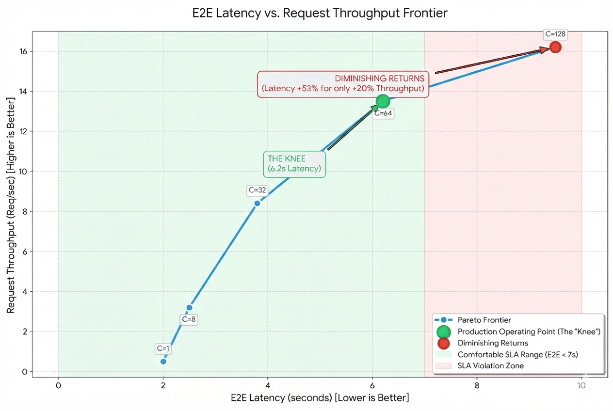
Step 2: Find the operating point

Every AI business and application is different and has unique performance needs. For example, specific e2e latency SLAs while keeping the cost-per-token low. So, how do you find the most optimal point on the frontier?

Start with the performance SLA as there’s usually some wiggle room in the latency SLAs—in other words, instead of a single number, target a range (if possible) that is acceptable for the use case. For most production workloads, the most “optimal” point isn’t at the absolute maximum throughput, but at the edge of your latency SLA. If your P99 latency is comfortably within your target range at Concurrency 64, but doubles at Concurrency 128 for only a 10% gain in throughput, C=64 is your production operating point**.**

Finding the operating point is where engineering meets unit economics. This is the art of finding the exact moment when the system starts thrashing, where you are extracting most value out of the hardware without impacting user experience.

Step 3: Push the Frontier

Benchmarking is not a one-time event, but a continuous process. Look for optimization techniques that can push the frontier up and to the left:

• Does moving to FP8 on your GPUs lower the ITL enough to let you double your batch size while staying in SLA?
• Can a small draft model with speculative decoding “cheat” the memory-bound nature of the decode phase to lower your TPOT?
• How do you maintain a profitable frontier with large context windows - e.g. > 128K?
• Can you “under-volt” the GPUs to get 90% of performance at 70% of the energy cost?
• For larger models, like Qwen3-235B, does running two TP4 groups than a single TP8 help to pack in more request density?

Answers to some of these questions involve modeling advanced frontiers for Quality vs Cost, Context Window vs Throughput, Power / Thermal vs Performance etc. Layering in the optimizations to push the frontiers has a direct impact on cost-per-token and TCO. As an example, in our work with character.ai, we were able to pack-in more request throughput by making optimal use of distributed parallelism strategies. From the frontier standpoint, this pushed the frontier UP—in other words, more throughput under similar e2e latency SLAs.

When in doubt, keep the speed of light frontier as the north star. This will keep you grounded as the software/kernel tax and comparing relative benchmarks from multiple sources often leave you more confused than providing a grounded truth from first principles.

Micro-benchmarks

So far, we focused mostly on end-to-end benchmarks with end to end metrics and user responsiveness. In many scenarios, the noise of the entire system is too much to isolate a specific issue. For example, if TTFT is 3x slower than expected, it could be because of several reasons. Micro-benchmarks aim to isolate and stress test a specific component. In the context of LLMs, micro-benchmarks help in finding bottlenecks in kernels, memory bandwidth, and interconnects.

Memory Bandwidth (HBM / SRAM)

Memory bandwidth benchmarks are useful to isolate TPOT slowness issues since decode is a memory-bound phase. Usually, the benchmarks can help isolate whether the performance is at-par with what is mentioned in the vendor’s specs.

Compute (GEMM) & Attention Kernels (Flash Attention, MHA, MLA etc)

These benchmarks help isolate performance issues with the attention kernels. One important point to note for compute and attention kernels is that it is extremely important to benchmark these kernels while moving across generations of GPUs. For example, a kernel written for A100 with 90% FLOPs utilization may drop to 30% utilization on an H100.

One reason for this is that every new compute generation changes the compute/bandwidth ratio. Usually, FLOPs increase faster than HBM bandwidth which can result in implications such as a kernel that was compute bound on an A100 becomes memory bound on an H100. Running the benchmarks again and tuning the kernels for the new hardware generation becomes a critical step to ensure you are squeezing the most performance from newer hardware generations.

In general, as an industry, we have a long way to go to achieve true software portability at the kernel level across hardware generations or vendors. To squeeze the most performance out of the hardware and have deterministic performance without power/thermal throttling, running a kernel sweep across the fleet, kernel tuning, and rigorously testing for optimal performance is the only way to go.

Collectives (NCCL / RCCL)

Large models that don’t fit into a single GPU memory usually run with parallelism topologies like Tensor Parallelism (TP), Pipeline Parallelism (PP), or Expert Parallelism (EP). These parallelism techniques rely on high speed GPU-to-GPU links within an 8x server or across servers over RDMA and utilize collectives like “all_reduce” (e.g. for TP) or “all_all” (e.g. for expert routing in MoE models with EP. MoE routing is particularly sensitive to interconnect latency) for optimal model serving.

Benchmarking collective and point-to-point performance intra node (NVlink, AMD Infinity Fabric) and multi-node (RDMA) is an absolute must. Moreover, test for both small and large messages. Large prompt prefills push large messages (32 MB - 1 GB+) through the interconnects, while the decode phase is more heavy on small messages (32 KB - 1 MB).

As an example, in the decode phase, TP performs “all_reduce” on very small activation vectors. Measure latency, algo, and bus bandwidth for a large sweep of message sizes (e.g. 1 MB - 16 GB). Even in the case of collective benchmarks, NIC (eg. 8 * 400 Gbps) / Intra server peak GPU-to-GPU provides a speed of light frontier but there is algorithm overhead which doesn’t let you go to peak bandwidth (and that is ok).

Measure What Matters: From the First Principles

By decomposing inference performance into its foundational building blocks, including metrics, FLOPs, memory bandwidth utilization, efficiency, and contention, AI teams can establish a baseline Pareto frontier by mapping these variables against a throughput and concurrency surface. This framework provides a rigorous methodology for identifying the optimal operating point for any given workload and serves as a grounded starting point for further optimization.

However, as inference scales, production teams must move beyond a single graph to identify additional frontiers, such as the Quality-Cost-Precision triad and the Power/Thermal vs Performance, to navigate the complex trade-offs between model quantization, accuracy, and unit economics. This requires a deep understanding of model architecture mapping to hardware, ensuring that specific structural choices like attention mechanisms or expert routing are precisely aligned with underlying hardware primitives to maximize the performance of the system.