A Review of Popular Deep Learning Architectures: AlexNet, VGG16, and GoogleNet

Introduction

Problems ranging from image recognition to image generation and tagging have benefited greatly from various deep learning (DL) architectural advancements. Understanding the intricacies of different DL models will help you understand the evolution of the field, and find the right fit for the problems you’re trying to solve.

Over the past couple of years many architectures have sprung up varying in many aspects, such as the types of layers, hyperparameters, etc. In this series we’ll review several of the most notable DL architectures that have defined the field and redefined our ability to tackle critical problems.

In the first part of this series we’ll cover “earlier” models that were published  from 2012 to 2014. This includes:

• AlexNet
• VGG16
• GoogleNet

Prerequisites

To fully grasp the concepts we highly recommend to have a basic understanding of deep learning and neural networks, specifically convolutional neural networks (CNNs). Familiarity with key concepts such as layers, activation functions, backpropagation, and gradient descent is needed. A general knowledge of image processing techniques and experience with a deep learning framework like TensorFlow or PyTorch will also be helpful for understanding the practical applications of these architectures.

AlexNet (2012)

AlexNet is one of the most popular neural network architectures to date. It was proposed by Alex Krizhevsky for the ImageNet Large Scale Visual Recognition Challenge (ILSVRV), and is based on convolutional neural networks. ILSVRV evaluates algorithms for Object Detection and Image Classification. In 2012, Alex Krizhevsky et al. published ImageNet Classification with Deep Convolutional Neural Networks. This is when AlexNet was first heard of.

The challenge was to develop a Deep Convolutional Neural Network to classify the 1.2 million high-resolution images in the ImageNet LSVRC-2010 dataset into more than 1000 different categories. The architecture achieved a top-5 error rate (the rate of not finding the true label of a given image among a model’s top-5 predictions) of 15.3%. The next best result trailed far behind at 26.2%.

AlexNet Architecture

The architecture is comprised of eight layers in total, out of which the first 5 are convolutional layer and the last 3 are fully-connected. The first two convolutional layers are connected to overlapping max-pooling layers to extract a maximum number of features. The third, fourth, and fifth convolutional layers are directly connected to the fully-connected layers. All the outputs of the convolutional and fully-connected layers are connected to ReLu non-linear activation function. The final output layer is connected to a softmax activation layer, which produces a distribution of 1000 class labels.

AlexNet Architecture

The input dimensions of the network are (256 × 256 × 3), meaning that the input to AlexNet is an RGB (3 channels) image of (256 × 256) pixels. There are more than 60 million parameters and 650,000 neurons involved in the architecture. To reduce overfitting during the training process, the network uses dropout layers. The neurons that are “dropped out” do not contribute to the forward pass and do not participate in backpropagation. These layers are present in the first two fully-connected layers.

AlexNet Training and Results

The model uses a stochastic gradient descent optimization function with batch size, momentum, and weight decay set to 128, 0.9, and 0.0005 respectively. All the layers use an equal learning rate of 0.001. To address overfitting during training, AlexNet uses both data augmentation and dropout layers. It took approximately six days to train on two GTX 580 3GB GPUs for 90 cycles.

Below is a screenshot of the results that were obtained using the AlexNet Architecture:

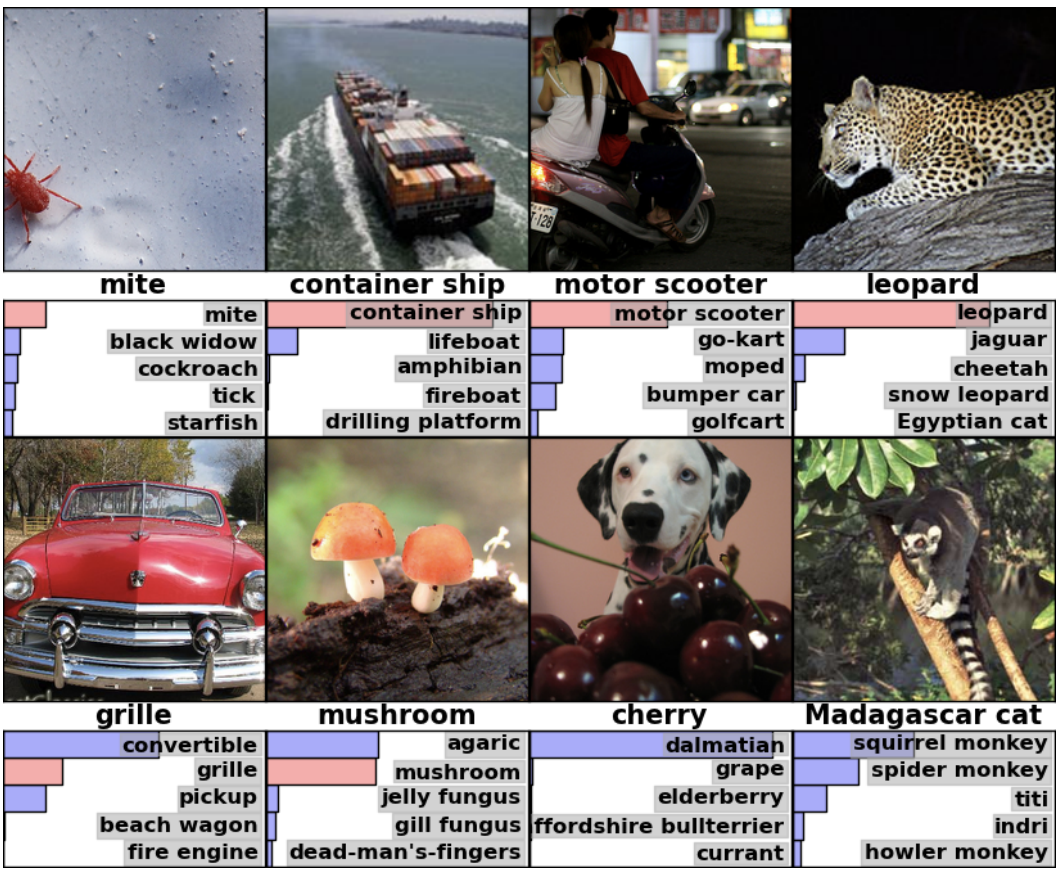
Results Using AlexNet on the ImageNet Dataset

Regarding the results on the ILSVRC-2010 dataset, AlexNet achieved top-1 and top-5 test set error rates of 37.5% and 17.0% when the competition was held.

Popular deep learning frameworks like PyTorch and TensorFlow now have the basic implementation of architectures like AlexNet. Below are a few relevant links for implementing it on your own.

1. Tensorflow AlexNet Model
2. Other references: Understanding AlexNet
3. The original paper: ImageNet Classification with Deep Convolutional Neural Networks

VGG16 (2014)

VGG is a popular neural network architecture proposed by Karen Simonyan & Andrew Zisserman from the University of Oxford. It is also based on CNNs, and was applied to the ImageNet Challenge in 2014. The authors detail their work in their paper, Very Deep Convolutional Networks for large-scale Image Recognition. The network achieved 92.7% top-5 test accuracy on the ImageNet dataset.

Major improvements of VGG, when compared to AlexNet, include using large kernel-sized filters (sizes 11 and 5 in the first and second convolutional layers, respectively) with multiple (3×3) kernel-sized filters, one after another.

VGG Architecture

The input dimensions of the architecture are fixed to the image size, (244 × 244). In a pre-processing step the mean RGB value is subtracted from each pixel in an image.

Source: Step by step VGG16 implementation in Keras for beginners

After the pre-processing is complete the images are passed to a stack of convolutional layers with small receptive-field filters of size (3×3). In a few configurations the filter size is set to (1 × 1), which can be identified as a linear transformation of the input channels (followed by non-linearity).

The stride for the convolution operation is fixed to 1. Spatial pooling is carried out by five max-pooling layers, which follow several convolutional layers. The max-pooling is performed over a (2 × 2) pixel window, with stride size set to 2.

The configuration for fully-connected layers is always the same; the first two layers have 4096 channels each, the third performs 1000-way ILSVRC classification (and thus contains 1000 channels, one for each class), and the final layer is the softmax layer. All the hidden layers for the VGG network are followed by the ReLu activation function.

VGG Configuration, Training, and Results

The VGG network has five configurations named A to E. The depth of the configuration increases from left (A) to right (B), with more layers added. Below is a table describing all the potential network architectures:

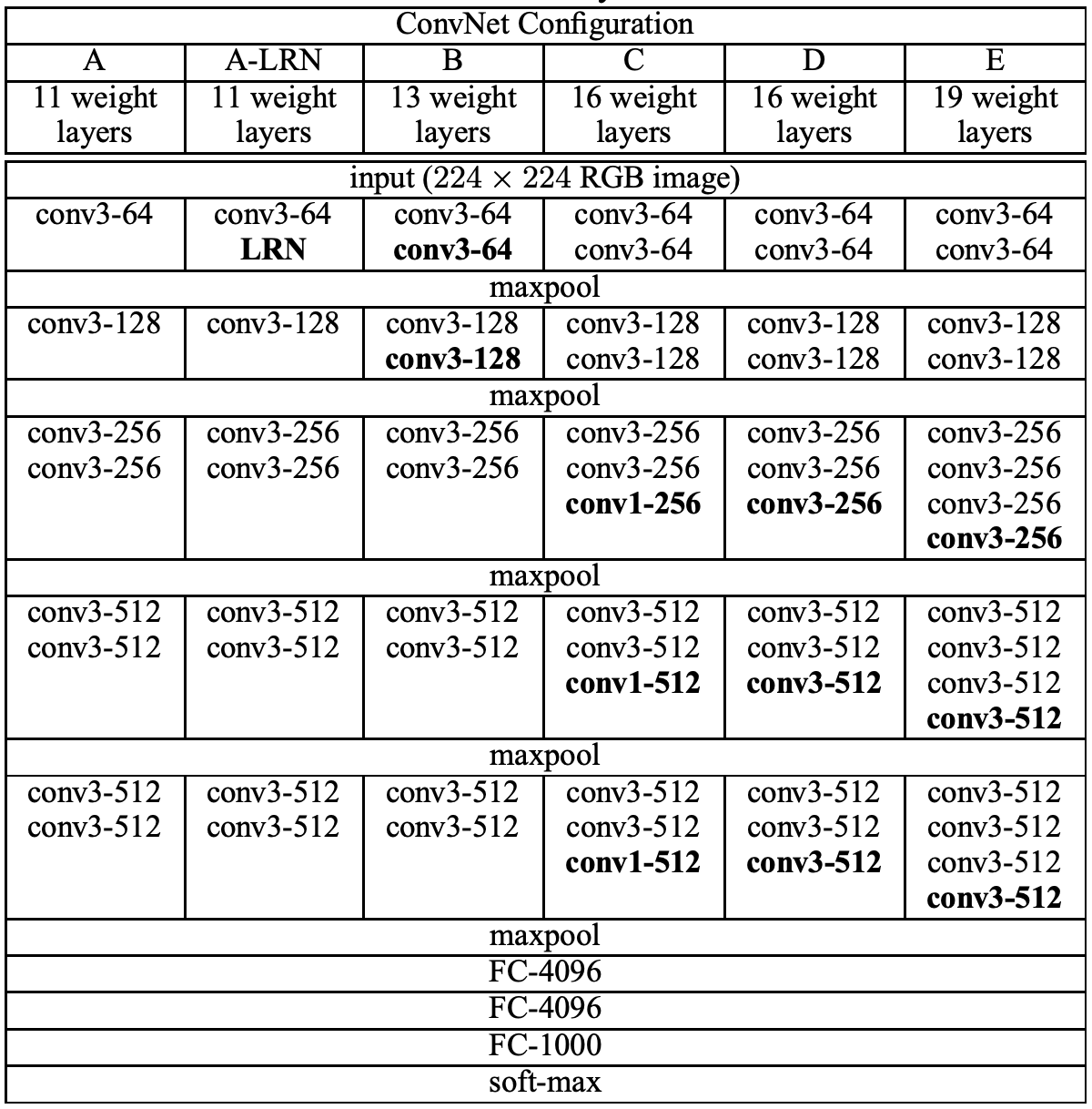
All configurations follow the universal pattern in architecture and differ only in depth; from 11 weight layers in network A (8 convolutional and 3 fully-connected layers), to 19 weight layers in network E (16 convolutional and 3 fully-connected layers). The number of channels of convolutional layers is rather small, starting from 64 in the first layer and then increasing by a factor of 2 after each max-pooling layer, until reaching 512. Below is an image showing the total number of parameters (in millions):

Training an image on the VGG network uses techniques similar to Krizhevsky et al., mentioned previously (i.e. the training of AlexNet). There are only a few exceptions when multi-scale training images are involved. The entire training process is carried out by optimizing the multinomial logistic regression objective using mini-batch gradient descent based on backpropagation. The batch size and the momentum are set to 256 and 0.9, respectively. The dropout regularization was added for the first two fully-connected layers setting the dropout ratio to 0.5. The learning rate of the network was initially set to 0.001 and then decreased by a factor of 10 when the validation set accuracy stopped improving. In total, the learning rate was reduced 3 times, and the learning was stopped after 370,000 iterations (74 epochs).

VGG16 significantly outperformed the previous generation of models in both the ILSVRC-2012 and ILSVRC-2013 competitions. Concerning the single-net performance, the VGG16 architecture achieved the best result (7.0% test error). Below is a table showing the error rates.

Regarding the hardware and training time, the VGG network took weeks of training using NVIDIA’s Titan Black GPUs.

There are two key drawbacks worth noting if you’re working with a VGG network. First, it takes a lot of time to train. Second, the network architecture weights are quite large. Due to its depth and number of fully-connected nodes, the trained VGG16 model is over 500MB. VGG16 is used in many deep learning image classification problems; however, smaller network architectures are often more desirable (such as SqueezeNet, GoogleNet, etc.)

Popular deep learning frameworks like PyTorch and TensorFlow have the basic implementation of the VGG16 architecture. Below are a few relevant links.

1. PyTorch VGG Implementation
2. Tensorflow VGG Implementation
3. Link to the Original Research Paper

GoogleNet (2014)

The Inception Network was one of the major breakthroughs in the fields of Neural Networks, particularly for CNNs. So far there are three versions of Inception Networks, which are named Inception Version 1, 2, and 3. The first version entered the field in 2014, and as the name “GoogleNet” suggests, it was developed by a team at Google. This network was responsible for setting a new state-of-the-art for classification and detection in the ILSVRC. This first version of the Inception network is referred to as GoogleNet.

If a network is built with many deep layers it might face the problem of overfitting. To solve this problem, the authors in the research paper Going deeper with convolutions proposed the GoogleNet architecture with the idea of having filters with multiple sizes that can operate on the same level. With this idea, the network actually becomes wider rather than deeper. Below is an image showing a Naive Inception Module.

As can be seen in the above diagram, the convolution operation is performed on inputs with three filter sizes: (1 × 1), (3 × 3), and (5 × 5). A max-pooling operation is also performed with the convolutions and is then sent into the next inception module.

Since neural networks are time-consuming and expensive to train, the authors limit the number of input channels by adding an extra (1 × 1) convolution before the (3 × 3) and (5 × 5) convolutions to reduce the dimensions of the network and perform faster computations. Below is an image showing a Naive Inception Module with this addition.

These are the building blocks of GoogleNet. Below is a detailed report on its architecture.

GoogleNet Architecture

The GoogleNet Architecture is 22 layers deep, with 27 pooling layers included. There are 9 inception modules stacked linearly in total. The ends of the inception modules are connected to the global average pooling layer. Below is a zoomed-out image of the full GoogleNet architecture.

The Orange Box in the architecture is the stem that has few preliminary convolutions. The purple boxes are the auxiliary classes. (Image Credits: A Simple Guide to the Versions of the Inception Network).

The detailed architecture and parameters are explained in the image below.

GoogleNet Training and Results

GoogleNet is trained using distributed machine learning systems with a modest amount of model and data parallelism. The training used asynchronous stochastic gradient descent with a momentum of 0.9 and a fixed learning rate schedule decreasing the learning rate by 4% every 8 epochs. Below is an image of the results of the teams that performed for ILSVRC 2014. GoogleNet stood in first place with an error rate of 6.67%.

Below are a few relevant links I encourage you to check out if you’re interested using or implementing GoogleNet.

1. Link to Original Research Paper
2. PyTorch Implementation of GoogleNet
3. Tensorflow Implementation of GoogleNet

Conclusion

These architectures have set the base for many of today’s advanced deep learning models. Introduction to AlexNet and the use of GPUs marked a turning point in image classification performance. VGG16 demonstrated the power of depth and simplicity by utilizing small convolutional filters, while GoogleNet introduced the Inception module to achieve a balance between efficiency and accuracy.