Tutorial

Deep Learning Architecture Review: DenseNet, ResNeXt, MnasNet & ShuffleNet v2

Updated on March 3, 2025

Deep Learning Architecture Review: DenseNet, ResNeXt, MnasNet & ShuffleNet v2

Introduction

This article takes a closer look at some of the most influential deep learning models that have shaped the field and made it easier to tackle complex problems. We’ll explore how these architectures improve efficiency and accuracy, making AI more powerful and accessible. The models we’ll cover include:

DenseNet
ResNeXt
MnasNet
ShuffleNet v2

Prerequisites

Basics of Convolutional Neural Networks (CNNs): Understanding how CNNs work, including concepts like convolutional layers, pooling layers, and fully connected layers.
Neural Network Training: Familiarity with backpropagation, optimization techniques (e.g., SGD, Adam), and loss functions.
Model Evaluation Metrics: Knowledge of metrics such as accuracy, precision, recall, and F1-score to evaluate the performance of deep learning models.
Understanding of Transfer Learning: Basics of transfer learning and how pre-trained models can be fine-tuned for specific tasks.
Residual Connections: Awareness of the concept of residual connections as introduced in ResNet, which helps in understanding the advancements in models like ResNeXt.

DenseNet (2016)

The name “DenseNet” refers to Densely Connected Convolutional Networks. It was proposed by Gao Huang, Zhuang Liu, and their team in 2017 at the CVPR Conference.

Traditional convolutional networks with n number of layers have n deep connections, one between each layer and its subsequent layer. In DenseNet, each layer connects to every other layer in a feed-forward fashion, meaning that DenseNet has n(n+1)/2 connections. For each layer, the feature maps of all preceding layers are used as inputs, and its feature-maps are used as inputs to all subsequent layers.

Dense Blocks

DenseNet boasts one big advantage over conventional deep CNNs: the information passed through many layers will not be washed out or vanish when it reaches the network’s end. A simple connectivity pattern achieves this. To understand this, one must know how layers in a normal CNN are connected.

Here’s a simple CNN where the layers are sequentially connected. In the Dense Block, however, each layer obtains additional inputs from all preceding layers, and passes its own feature maps to all subsequent layers. Below is an image depicting the dense block.

As the layers in the network receive feature maps from all the preceding layers, the network will be thinner and more compact. Below is a 5-layer dense block with the number of channels set to 4.

The DenseNet Architecture

DenseNet has been applied to various different datasets. Based on the dimensionality of the input, different types of dense blocks are used. Below is a brief description of these layers. Basic DenseNet Composition Layer: In this type of dense block each layer is followed by a pre-activated batch normalization layer, ReLU activation function, and a 3×3 convolution. Below is a snapshot.

BottleNeck DenseNet (DenseNet-B): As every layer produces k output feature maps, computation can be harder at every level. Hence the authors presented a bottleneck structure where 1×1 convolutions are used before a 3×3 convolution layer, shown below.

DenseNet Compression: To improve the model compactness, the authors tried reducing the feature maps at the transition layers. So if a dense block consists of m feature maps and the transition layer generates i output feature maps, where 0 < i <= 1, this i also denotes the compression factor. If the value of i is equal to one (i=1), the number of feature maps across transition layers remains unchanged. If i < 1, then the architecture is referred to as DenseNet-C and the value of i would be changed to 0.5. When both the bottleneck and transition layers with i < 1 are used, we refer to our model as DenseNet-BC.

Multiple Dense Blocks with Transition Layers: The dense blocks in the architecture are followed by a 1×1 Convolution layer and 2×2 average pooling layer. As the feature map sizes are the same, it’s easy to concatenate the transition layers. Lastly, at the end of the dense block, a global average pooling is performed which is attached to a softmax classifier.

DenseNet Training and Results

The DenseNet architecture defined in the original research paper is applied to three datasets: CIFAR, SVHN, and ImageNet. All the architectures used a stochastic gradient descent optimizer for training. The training batch size for CIFAR and SVHN was 64, for 300 and 40 epochs, respectively. The initial learning rate was set to 0.1 and was further reduced. Below are the metrics for DenseNet trained on ImageNet:

Batch size: 256
Epochs: 90
Learning rate: 0.1, decreased by a factor of 10 at epochs 30 and 60
Weight decay and momentum: 0.00004 and 0.9

Below are the detailed results showing how different configurations of DenseNet compare to other networks on the CIFAR and SVHN datasets. The data in blue indicates the best results.

Below are the Top-1 and Top-5 errors for different sizes of DenseNet on ImageNet.

Here are some useful links if you’d like to explore the original paper, check out its implementation, or learn how to use DenseNet yourself:

Most of the images in this review are taken from the original research paper (DenseNet) and the article Review: DenseNet — Dense Convolutional Network (Image Classification) by Sik-Ho Tsang
Code corresponding to the original paper
TensorFlow Implementation of DenseNet
PyTorch Implementation of DenseNet

ResNeXt (2017)

ResNeXt is a homogeneous neural network which reduces the number of hyperparameters required by conventional ResNet. This is achieved by their use of “cardinality”, an additional dimension on top of the width and depth of ResNet. Cardinality defines the size of the set of transformations.

In this image the leftmost diagram is a conventional ResNet block; the rightmost is the ResNeXt block, which has a cardinality of 32. The same transformations are applied 32 times, and the result is aggregated at the end. This technique was suggested in the 2017 paper Aggregated Residual Transformations for Deep Neural Networks, co-authored by Saining Xie, Ross Girshick, Piotr Dollar, Zhuowen Tu, and Kaiming He, who all worked under Facebook AI Research.

VGG-nets, ResNets, and Inception Networks have gained a lot of momentum in the field of feature engineering. Despite their great performances, they still face a handful of limitations. These models are well-suited for several datasets, but due to the many hyperparameters and computations involved, adapting them to new datasets is no minor task. To overcome such issues, the advantages of both VGG/ResNet (ResNet evolved from VGG) and Inception Networks have been considered. In a nutshell, the repetition strategy of ResNet is combined with the split-transform-merge strategy of Inception Network. In other words, a network block splits the input, transforms it into a required format, and merges it to get the output where each block follows the same topology.

ResNeXt Architecture

The basic architecture of ResNeXt is defined by two rules. First, if the blocks produce same-dimensional spatial maps, they share the same set of hyperparameters, and if at all the spatial map is downsampled by a factor of 2, the width of the block is multiplied by a factor of 2.

As seen in the table, ResNeXt-50 has 32 as its cardinality repeated 4 times (depth). The dimensions in [] denote the residual block structures, whereas the numbers written adjacent to them refer to the number of stacked blocks. 32 precisely denotes that there are 32 groups in the grouped convolution.

The above network structures explain what a grouped convolution is, and how it trumps the other two network structures.

(a) denotes a usual ResNeXt block that has already been seen previously. It has a cardinality of 32, and follows the split-transform-merge strategy. (b) does seem to be a leaf taken out of Inception-ResNet. However, Inception or Inception-ResNet doesn’t have network blocks following the same topology. © is related to the grouped convolution which has been proposed in AlexNet architecture. 32*4 as has been seen in (a) and (b) has been replaced with 128 in-short, meaning splitting is done by a grouped convolutional layer. Similarly, the transformation is done by the other grouped convolutional layer that does 32 groups of convolutions. Later, concatenation happens.

Among the above three, © proved to be the best as it is simple to implement.

ResNeXt Training and Results

ImageNet has been used to show the enhancement in accuracy when cardinality is considered rather than width/depth.

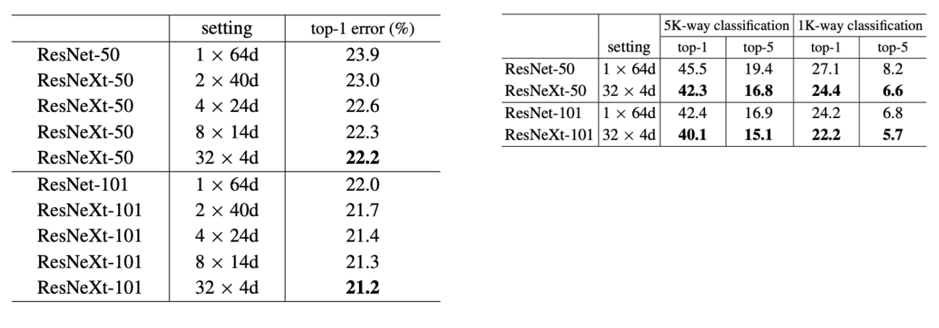
Both ResNeXt-50 and ResNeXt-101 are less error-prone when the cardinality is high. Also, in comparison to ResNet, ResNeXt performed well. If you want to dive deeper into DenseNet, there are several valuable resources to explore. The original research paper provides a detailed explanation of its architecture and how it improves feature reuse to enhance deep learning performance. For those interested in practical implementation, the official ResNext site offers code examples.

ShuffleNet v2 (2018)

ShuffleNet v2 considers direct metrics, such as speed or memory access cost, to measure the network’s computational complexity (besides FLOPs, which acts as an indirect metric). Moreover, the direct metrics are also evaluated on the target platform. ShuffleNet v2 was thus introduced in the paper, ShuffleNet V2: Practical Guidelines for Efficient CNN Architecture Design, published in 2018. It was co-authored by Ningning Ma, Xiangyu Zhang, Hai-Tao Zheng, and Jian Sun.

FLOPs is the usual metric to measure the performance of a network, in terms of its computations. However, a few studies have substantiated the fact that FLOPs do not wholly dig the underlying truths; networks having similar FLOPs differ in their speeds, this can be because of the memory access cost, degree of parallelism, target platform, etc. All these do not fall under FLOPs, and thus, are being ignored. ShuffleNet v2 overcomes such hassles by proposing four guidelines to model a network.

ShuffleNet v2 Architecture

Prior to understanding the network architecture, the guidelines upon which the network has been built shall give a glimpse into how various other direct metrics have been considered:

Equal channel width minimizes the memory access cost: When the number of input channels and output channels are in the same proportion (1:1), memory access cost becomes low.
Excessive group convolution increases memory access cost: The group number shouldn’t be too high, otherwise the memory access cost tends to increase.
Network fragmentation reduces degree of parallelism: Fragmentation reduces the network’s efficiency in executing parallel computations.
Element-wise operations are non-negligible: Element-wise operations have small FLOPs, but can increase the memory access time.

All these are integrated in the ShuffleNet v2 architecture to improve the network efficiency.

The channel split operator divides the channels into two groups, where one remains as an identity (3rd guideline). The other branch has an equal number of input and output channels along the three convolutions (1st guideline). The 1x1 convolutions aren’t group-wise (2nd guideline). Element-wise operations like ReLU, Concat, depth-wise convolutions are confined to a single branch (4the guideline).

The overall ShuffleNet v2 architecture is tabulated as follows:

The results are with respect to different variations of the output channels.

ShuffleNet v2 Training and Results

Imagenet has been used as the dataset to derive results with various datasets.

Complexity, error rate, GPU speed, and ARM speed have been used to derive the robust and efficient model among the contemplated models. Although ShuffleNet v2 lacks GPU speed, it records the lowest top-1 error rate, which outweighs the other limitations.

If you’re interested in learning more about ShuffleNet v2, here are some valuable resources to explore. The original research paper provides an in-depth explanation of the architecture, highlighting its efficiency in computational cost and accuracy for mobile and edge devices. If you’re looking to implement ShuffleNet v2, you can check out the TensorFlow implementation for a structured approach using Google’s deep learning framework. Alternatively, if you prefer PyTorch, the PyTorch implementation offers a practical guide to integrating ShuffleNet v2 into your projects. Whether you’re diving into the theory or experimenting with the model, these resources will help you get started.

MnasNet (2019)

MnasNet is an automated mobile neural architecture search network that is used to build mobile models using reinforcement learning. It incorporates the basic essence of CNN and thereby strikes the right balance between enhancing accuracy and reducing latency to depict high performance when the model is deployed onto a mobile. This idea was put forth in the paper, MnasNet: Platform-Aware Neural Architecture Search for Mobile, which was released in 2019. It was co-authored by Mingxing Tan, Bo Chen, Ruoming Pang, Vijay Vasudevan, Mark Sandler, Andrew Howard, and Andrew Howard–all belonging to the Google Brain team.

The conventional mobile CNN models developed so far do not yield the right outcome when latency and accuracy are taken into account; they somehow lack either of those. The latency is often estimated using FLOPS, which doesn’t output the right results. However, in MnasNet, the model is directly deployed onto a mobile, and the results are estimated; no proxies are involved. Mobiles are usually resource-constrained. Therefore, factors such as performance, cost, and latency are significant metrics to be considered.

MnasNet Architecture

The architecture generally consists of two phases - search space and reinforcement learning approach.

Factorized hierarchical search space: The search space supports diverse layer structures to be included throughout the network. The CNN model is factorized into various blocks wherein each block has a unique layer architecture. The connections are chosen such that both the input and output are compatible with each other, and henceforth yield good results to maintain a higher accuracy rate. The following image represents a search space:

As can be noticed, there are several blocks that make-up for the search space. All the layers are segregated based on their dimensions and filter size. Each block has a specific set of layers where the operations are chosen (as mentioned in blue color). The first layer in every block has a stride 2 if input or output dimensions are different, and the stride is 1 for the remaining layers. The same set of operations is repeated starting from the second layer to the Nth layer where N is the block number.

Reinforcement search algorithm: As we have two major objectives to achieve - latency and accuracy, we employ a reinforcement learning approach where the rewards are maximized (multi-objective reward). Each CNN model as defined in the search space would be mapped to a sequence of actions that are to be performed by a reinforcement learning agent.

This is what is present in the search algorithm - the controller is a Recurrent Neural Network (RNN), and the trainer trains the model and outputs the accuracy. The model is deployed onto a mobile phone to estimate the latency. Both accuracy and latency are consolidated into a multi-objective reward. This reward is sent to RNN using which the parameters of RNN are updated, to maximize the total reward.

MnasNet Training and Results

Imagenet has been used to depict the accuracy achieved by a MnasNet model, in comparison with the other conventional mobile CNN models. Here’s a table representing the same:

MnasNet is designed to achieve both reduced latency and improved accuracy, making it highly efficient for mobile and edge devices. If you’d like to explore the model in more detail, you can read the original research paper to understand its architecture and optimization techniques. For hands-on implementation, check out the PyTorch implementation to integrate MnasNet into your projects.

Model	Pros	cons
DenseNet	- Efficient feature reuse through dense connections, reducing redundancy.	- Computationally expensive due to dense connectivity.
	- Fewer parameters compared to traditional CNNs, making it memory-efficient.	- Increased training time compared to ResNet.
	- Strong gradient flow due to shorter connections between layers.	- May not scale well for very deep networks.
ResNeXt	- Improved performance with grouped convolutions, leading to better accuracy.	- Higher memory and computation cost compared to ResNet.
	- More efficient than standard ResNet while maintaining similar model depth.	- More complex than standard CNNs, requiring careful hyperparameter tuning.
	- Scalable architecture with a modular design.
MnasNet	- Optimized for mobile devices with efficient hardware-aware architecture search.	- Designed primarily for mobile and edge devices, limiting flexibility for high-end tasks.
	- Provides a good balance between accuracy and latency.	- Requires specialized NAS (Neural Architecture Search) for optimization.
	- Achieves high performance with fewer computational resources.
ShuffleNet v2	- Highly efficient for mobile and edge computing due to lightweight design.	- Not as accurate as larger CNN models in complex tasks.
	- Uses channel split and shuffle operations to improve speed and efficiency.	- Optimization challenges when scaling for high-end applications.
	- Faster than previous ShuffleNet versions while maintaining accuracy.

Conclusion

Deep learning architectures like DenseNet, ResNeXt, MnasNet, and ShuffleNet v2 have significantly advanced the field by improving efficiency, accuracy, and scalability. Each model offers unique benefits, from DenseNet’s feature reuse to MnasNet’s mobile optimization. Understanding these architectures helps in selecting the right model for specific applications, whether it’s high-performance computing or edge AI deployment. As deep learning continues to evolve, these innovations pave the way for more efficient and accessible AI solutions.