PyTorch Loss Functions

Introduction

Loss functions are fundamental in ML model training, and, in most machine learning projects, there is no way to drive your model into making correct predictions without a loss function. In layman terms, a loss function is a mathematical function or expression used to measure how well a model is doing on some dataset. Knowing how well a model is doing on a particular dataset gives the developer insights into making a lot of decisions during training such as using a new, more powerful model or even changing the loss function itself to a different type. Speaking of types of loss functions, there are several of these loss functions which have been developed over the years, each suited to be used for a particular training task.

Prerequisites

This article requires understanding neural networks. At a high level, neural networks are composed of interconnected nodes (“neurons”) organized into layers. They learn and make predicitions through a process called “training” which adjusts the weights and biases of the connections between neurons. An understanding of neural networks includes knowledge of their different layers (input layer, hidden layers, output layer), activation functions, optimization algorithms (variants of gradient descent), loss functions, etc.

Additionally, familiarity with Python syntax and the PyTorch library is essential for understanding the code snippets presented in this article.

In this article, we are going to explore different loss functions which are part of the PyTorch nn module. We will further take a deep dive into how PyTorch exposes these loss functions to users as part of its nn module API by building a custom one.

Now that we have a high-level understanding of what loss functions are, let’s explore some more technical details about how loss functions work.

What are loss functions?

We stated earlier that loss functions tell us how well a model does on a particular dataset. Technically, how it does this is by measuring how close a predicted value is close to the actual value. When our model is making predictions that are very close to the actual values on both our training and testing dataset, it means we have a quite robust model.

Although loss functions give us critical information about the performance of our model, that is not the primary function of loss function, as there are more robust techniques to assess our models such as accuracy and F-scores. The importance of loss functions is mostly realized during training, where we nudge the weights of our model in the direction that minimizes the loss. By doing so, we increase the probability of our model making correct predictions, something which probably would not have been possible without a loss function.

Different loss functions suit different problems, each carefully crafted by researchers to ensure stable gradient flow during training.

Sometimes, the mathematical expressions of loss functions can be a bit daunting, and this has led to some developers treating them as black boxes. We are going to uncover some of PyTorch’s most used loss functions later, but before that, let us take a look at how we use loss functions in the world of PyTorch.

Loss functions in PyTorch

PyTorch comes out of the box with a lot of canonical loss functions with simplistic design patterns that allow developers to easily iterate over these different loss functions very quickly during training. All PyTorch’s loss functions are packaged in the nn module, PyTorch’s base class for all neural networks. This makes adding a loss function into your project as easy as just adding a single line of code. Let’s look at how to add a mean squared error loss function in PyTorch.

import torch.nn as nn
MSE_loss_fn = nn.MSELoss()

The function returned from the code above can be used to calculate how far a prediction is from the actual value using the format below.

#predicted_value is the prediction from our neural network
#target is the actual value in our dataset
#loss_value is the loss between the predicted value and the actual value
Loss_value = MSE_loss_fn(predicted_value, target)

Now that we have an idea of how to use loss functions in PyTorch, let’s dive deep into the behind the scenes of several of the loss functions PyTorch offers.

Which loss functions are available in PyTorch?

A lot of these loss functions PyTorch comes with are broadly categorised into 3 groups - regression loss, classification loss and ranking loss.

Regression losses are mostly concerned with continuous values which can take any value between two limits. One example of this would be predictions of the house prices of a community.

Classification loss functions deal with discrete values, like the task of classifying an object as a box, pen or bottle.

Ranking losses predict the relative distances between values. An example of this would be face verification, where we want to know which face images belong to a particular face, and can do so by ranking which faces do and do not belong to the original face-holder via their degree of relative approximation to the target face scan.

L1 loss function/ Mean Absolute Error

The L1 loss function computes the mean absolute error between each value in the predicted tensor and that of the target. It first calculates the absolute difference between each value in the predicted tensor and that of the target, and computes the sum of all the values returned from each absolute difference computation. Finally, it computes the average of this sum value to obtain the mean absolute error (MAE). The L1 loss function is very robust for handling noise.

import torch.nn as nn

#size_average and reduce are deprecated

#reduction specifies the method of reduction to apply to output. Possible values are 'mean' (default) where we compute the average of the output, 'sum' where the output is summed and 'none' which applies no reduction to output

Loss_fn = nn.L1Loss(size_average=None, reduce=None, reduction='mean')

input = torch.randn(3, 5, requires_grad=True)
target = torch.randn(3, 5)
output = loss_fn(input, target)
print(output) #tensor(0.7772, grad_fn=<L1LossBackward>)

The single value returned is the computed loss between two tensors with dimension 3 by 5.

Mean Squared Error

The mean squared error shares some striking similarities with MAE. Instead of computing the absolute difference between values in the prediction tensor and target, as is the case with mean absolute error, it computes the squared difference between values in the prediction tensor and that of the target tensor. By doing so, relatively large differences are penalized more, while relatively small differences are penalized less. MSE is considered less robust at handling outliers and noise than MAE, however.

import torch.nn as nn

loss = nn.MSELoss(size_average=None, reduce=None, reduction='mean')
#L1 loss function parameters explanation applies here.

input = torch.randn(3, 5, requires_grad=True)
target = torch.randn(3, 5)
output = loss(input, target)
print(output) #tensor(0.9823, grad_fn=<MseLossBackward>)

Cross-Entropy Loss

Cross-entropy loss is used in classification problems involving a number of discrete classes. It measures the difference between two probability distributions for a given set of random variables. Usually, when using cross-entropy loss, the output of our network is a softmax layer, which ensures that the output of the neural network is a probability value (value between 0-1).

The softmax layer consists of two parts - the exponent of the prediction for a particular class.

yi is the output of the neural network for a particular class. The output of this function is a number close to zero, but never zero, if yi is large and negative, and closer to 1 if yi is positive and very large.

import numpy as np

np.exp(34) #583461742527454.9
np.exp(-34) #1.713908431542013e-15

The second part is a normalization value and is used to ensure that the output of the softmax layer is always a probability value.

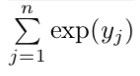
This is obtained by summing all the exponents of each class value. The final equation of softmax looks like this:

]

In PyTorch’s nn module, cross-entropy loss combines log-softmax and negative log-likelihood (NLL) loss into a single loss function.

Notice how the gradient function in the printed output is an NLL loss. This actually reveals that cross-entropy loss combines NLL loss under the hood with a log-softmax layer.

Negative Log-Likelihood (NLL) Loss

The NLL loss function works quite similarly to the cross-entropy loss function. Cross-entropy loss combines a log-softmax layer and NLL loss to obtain the value of the cross-entropy loss. This means that NLL loss can be used to obtain the cross-entropy loss value by having the last layer of the neural network be a log-softmax layer instead of a normal softmax layer.

m = nn.LogSoftmax(dim=1)
loss = nn.NLLLoss()
# input is of size N x C = 3 x 5
input = torch.randn(3, 5, requires_grad=True)
# each element in target has to have 0 <= value < C
target = torch.tensor([1, 0, 4])
output = loss(m(input), target)
output.backward()
# 2D loss example (used, for example, with image inputs)
N, C = 5, 4
loss = nn.NLLLoss()
# input is of size N x C x height x width
data = torch.randn(N, 16, 10, 10)
conv = nn.Conv2d(16, C, (3, 3))
m = nn.LogSoftmax(dim=1)
# each element in target has to have 0 <= value < C
target = torch.empty(N, 8, 8, dtype=torch.long).random_(0, C)
output = loss(m(conv(data)), target)
print(output) #tensor(1.4892, grad_fn=<NllLoss2DBackward>)

#credit NLLLoss — PyTorch 1.9.0 documentation

Binary Cross-Entropy Loss

Binary cross-entropy loss is a special class of cross-entropy losses used for the special problem of classifying data points into only two classes. Labels for this type of problem are usually binary, and our goal is therefore to push the model to predict a number close to zero for a zero label and a number close to one for a one label. Usually when using BCE loss for binary classification, the output of the neural network is a sigmoid layer to ensure that the output is either a value close to zero or a value close to one.

import torch.nn as nn

m = nn.Sigmoid()
loss = nn.BCELoss()
input = torch.randn(3, requires_grad=True)
target = torch.empty(3).random_(2)
output = loss(m(input), target)
print(output) #tensor(0.4198, grad_fn=<BinaryCrossEntropyBackward>)

Binary Cross-Entropy Loss with Logits

We mentioned in the previous section that a binary cross-entropy loss is usually output as a sigmoid layer to ensure that output is between 0 and 1. A binary cross-entropy loss with logits combines these two layers into just one layer. According to the PyTorch documentation, this is a more numerically stable version as it takes advantage of the log-sum exp trick.

import torch
import torch.nn as nn

target = torch.ones([10, 64], dtype=torch.float32)  # 64 classes, batch size = 10
output = torch.full([10, 64], 1.5)  # A prediction (logit)
pos_weight = torch.ones([64])  # All weights are equal to 1
criterion = torch.nn.BCEWithLogitsLoss(pos_weight=pos_weight)
loss = criterion(output, target)  # -log(sigmoid(1.5))
print(loss) #tensor(0.2014)

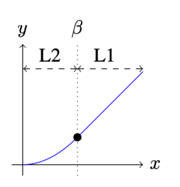
Smooth L1 Loss

The smooth L1 loss function combines the benefits of MSE loss and MAE loss through a heuristic value beta. This criterion was introduced in the Fast R-CNN paper. When the absolute difference between the ground truth value and the predicted value is below beta, the criterion uses a squared difference, much like MSE loss. The graph of MSE loss is a continuous curve, which means the gradient at each loss value varies and can be derived everywhere. Moreover, as the loss value reduces the gradient diminishes, which is convenient during gradient descent. However for very large loss values the gradient explodes, hence the criterion for switching to MAE, for which the gradient is almost constant for every loss value, when the absolute difference becomes larger than beta and the potential gradient explosion is eliminated.

import torch.nn as nn

loss = nn.SmoothL1Loss()
input = torch.randn(3, 5, requires_grad=True)
target = torch.randn(3, 5)
output = loss(input, target)

print(output) #tensor(0.7838, grad_fn=<SmoothL1LossBackward>)

Hinge Embedding Loss

Hinge embedding loss is mostly used in semi-supervised learning tasks to measure the similarity between two inputs. It’s used when there is an input tensor and a label tensor containing values of 1 or -1. It is mostly used in problems involving non-linear embeddings and semi-supervised learning.

import torch
import torch.nn as nn

input = torch.randn(3, 5, requires_grad=True)
target = torch.randn(3, 5)

hinge_loss = nn.HingeEmbeddingLoss()
output = hinge_loss(input, target)
output.backward()

print('input: ', input)
print('target: ', target)
print('output: ', output)

#input:  tensor([[ 1.4668e+00,  2.9302e-01, -3.5806e-01,  1.8045e-01,  #1.1793e+00],
#       [-6.9471e-05,  9.4336e-01,  8.8339e-01, -1.1010e+00,  #1.5904e+00],
#       [-4.7971e-02, -2.7016e-01,  1.5292e+00, -6.0295e-01,  #2.3883e+00]],
#       requires_grad=True)
#target:  tensor([[-0.2386, -1.2860, -0.7707,  1.2827, -0.8612],
#        [ 0.6747,  0.1610,  0.5223, -0.8986,  0.8069],
#        [ 1.0354,  0.0253,  1.0896, -1.0791, -0.0834]])
#output:  tensor(1.2103, grad_fn=<MeanBackward0>)

Margin Ranking Loss

Margin ranking loss belongs to the ranking losses whose main objective, unlike other loss functions, is to measure the relative distance between a set of inputs in a dataset. The margin ranking loss function takes two inputs and a label containing only 1 or -1. If the label is 1, then it is assumed that the first input should have a higher ranking than the second input and if the label is -1, it is assumed that the second input should have a higher ranking than the first input. This relationship is shown by the equation and code below.

import torch.nn as nn

loss = nn.MarginRankingLoss()
input1 = torch.randn(3, requires_grad=True)
input2 = torch.randn(3, requires_grad=True)
target = torch.randn(3).sign()
output = loss(input1, input2, target)
print('input1: ', input1)
print('input2: ', input2)
print('output: ', output)

#input1:  tensor([-1.1109,  0.1187,  0.9441], requires_grad=True)
#input2:  tensor([ 0.9284, -0.3707, -0.7504], requires_grad=True)
#output:  tensor(0.5648, grad_fn=<MeanBackward0>)

Triplet Margin Loss

This criterion measures similarity between data points by using triplets of the training data sample. The triplets involved are an anchor sample, a positive sample and a negative sample. The objective is 1) to get the distance between the positive sample and the anchor as minimal as possible, and 2) to get the distance between the anchor and the negative sample to have greater than a margin value plus the distance between the positive sample and the anchor. Usually, the positive sample belongs to the same class as the anchor, but the negative sample does not. Hence, by using this loss function, we aim to use triplet margin loss to predict a high similarity value between the anchor and the positive sample and a low similarity value between the anchor and the negative sample.

import torch.nn as nn

triplet_loss = nn.TripletMarginLoss(margin=1.0, p=2)
anchor = torch.randn(100, 128, requires_grad=True)
positive = torch.randn(100, 128, requires_grad=True)
negative = torch.randn(100, 128, requires_grad=True)
output = triplet_loss(anchor, positive, negative)
print(output)  #tensor(1.1151, grad_fn=<MeanBackward0>)

Cosine Embedding Loss

Cosine embedding loss measures the loss given inputs x1, x2, and a label tensor y containing values 1 or -1. It is used for measuring the degree to which two inputs are similar or dissimilar.

The criterion measures similarity by computing the cosine distance between the two data points in space. The cosine distance correlates to the angle between the two points which means that the smaller the angle, the closer the inputs and hence the more similar they are.

import torch.nn as nn

loss = nn.CosineEmbeddingLoss()
input1 = torch.randn(3, 6, requires_grad=True)
input2 = torch.randn(3, 6, requires_grad=True)
target = torch.randn(3).sign()
output = loss(input1, input2, target)
print('input1: ', input1)
print('input2: ', input2)
print('output: ', output)

#input1:  tensor([[ 1.2969e-01,  1.9397e+00, -1.7762e+00, -1.2793e-01, #-4.7004e-01,
#         -1.1736e+00],
#        [-3.7807e-02,  4.6385e-03, -9.5373e-01,  8.4614e-01, -1.1113e+00,
#          4.0305e-01],
#        [-1.7561e-01,  8.8705e-01, -5.9533e-02,  1.3153e-03, -6.0306e-01,
#          7.9162e-01]], requires_grad=True)
#input2:  tensor([[-0.6177, -0.0625, -0.7188,  0.0824,  0.3192,  1.0410],
#        [-0.5767,  0.0298, -0.0826,  0.5866,  1.1008,  1.6463],
#        [-0.9608, -0.6449,  1.4022,  1.2211,  0.8248, -1.9933]],
#       requires_grad=True)
#output:  tensor(0.0033, grad_fn=<MeanBackward0>)

Kullback-Leibler Divergence Loss

Given two distributions, P and Q, Kullback-Leibler (KL) divergence loss measures how much information is lost when P (assumed to be the true distributions) is replaced with Q. By measuring how much information is lost when we use Q to approximate P, we are able to obtain the similarity between P and Q and hence drive our algorithm to produce a distribution very close to the true distribution, P. The information loss when Q is used to approximate P is not the same when P is used to approximate Q, and thus KL divergence is not symmetric.

import torch.nn as nn

loss = nn.KLDivLoss(size_average=None, reduce=None, reduction='mean', log_target=False)
input1 = torch.randn(3, 6, requires_grad=True)
input2 = torch.randn(3, 6, requires_grad=True)
output = loss(input1, input2)

print('output: ', output) #tensor(-0.0284, grad_fn=<KlDivBackward>)

Building A Custom Loss Function

PyTorch provides us with two popular ways to build our own loss function to suit our problem; these are namely using a class implementation and using a function implementation. Let’s see how we can implement both methods starting with the function implementation.

This is easily the simplest way to write your own custom loss function. It’s just as easy as creating a function, passing into it the required inputs and other parameters, performing some operation using PyTorch’s core API or Functional API, and returning a value. Let’s see a demonstration with custom mean squared error.

def custom_mean_square_error(y_predictions, target):
  square_difference = torch.square(y_predictions - target)
  loss_value = torch.mean(square_difference)
  return loss_value

In the code above, we define a custom loss function to calculate the mean squared error given a prediction tensor and a target tensor

y_predictions = torch.randn(3, 5, requires_grad=True);
target = torch.randn(3, 5)
pytorch_loss = nn.MSELoss();
p_loss = pytorch_loss(y_predictions, target)
loss = custom_mean_square_error(y_predictions, target)
print('custom loss: ', loss)
print('pytorch loss: ', p_loss)

#custom loss:  tensor(2.3134, grad_fn=<MeanBackward0>)
#pytorch loss:  tensor(2.3134, grad_fn=<MseLossBackward>)

We can compute the loss using our custom loss function and PyTorch’s MSE loss function to observe that we have obtained the same results.

Custom Loss with Python Classes

This approach is probably the standard and recommended method of defining custom losses in PyTorch. The loss function is created as a node in the neural network graph by subclassing the nn module. This means that our custom loss function is a PyTorch layer exactly the same way a convolutional layer is. Let’s see a demonstration of how this works with a custom MSE loss.

class Custom_MSE(nn.Module):
  def __init__(self):
    super(Custom_MSE, self).__init__();

  def forward(self, predictions, target):
    square_difference = torch.square(predictions - target)
    loss_value = torch.mean(square_difference)
    return loss_value
  
  def __call__(self, predictions, target):
     square_difference = torch.square(y_predictions - target)
     loss_value = torch.mean(square_difference)
     return loss_value

Final Thoughts

We have discussed a lot about loss functions available in PyTorch and also taken a deep dive into the inner workings of most of these loss functions. Choosing the right loss function for a particular problem can be an overwhelming task. Hopefully, this tutorial alongside the official PyTorch documentation serves as a guideline when trying to understand which loss function suits your problem well.